How I Proved I was Unlucky using Cuda and Verified it with Math
First, a Small Disclaimer
This project started as curiosity-driven exploration without version control — I wanted to quantify just how absurd one particular game of Risk was. Many code snippets here are reconstructed to clearly show the progression of ideas, though the final results are fresh runs.
I thought it was an article worth writing for a few reasons:
- It’s funny, quantitative, and unique
- I think graphics-card (GPU) coding is cool, and this was an excuse to dive into some CUDA
- There is some cool math behind the theoretical model I came up with to validate my simulations
- It gives me an opportunity to use Latex on my blog
- It demonstrates work I’ve done and find cool
- Hopefully the reader will gain some sympathy for my pathological misfortune, and — perhaps — an unusually deep understanding of probabilities in Risk
The Motivation
People don’t take it seriously when I say I’m unlucky (I mean, fair, they shouldn’t). Especially if you have any experience with probability, you know that statistical improbabilities happen all the time. A one-off example doesn’t really mean someone is unlucky. Here are some grievances I have with Lady Luck:
- I had 3 strokes before the age of 30, one of them while on blood thinners
- When driving, every traffic light turns red as I approach a disproportionately high percentage of the time (like 80-90%)
- When playing D&D very consistently I will roll nat 20s when it doesn’t matter (animal handling an Ochre Jelly, initiative), and sub-10 when it matters a lot (an attack roll against a 1hp boss about to wipe our party)
- When playing Magic: The Gathering I consistently flood out drawing 15+ lands in 20 cards while running card draw engines, or get mana screwed on 2 lands for 8 turns straight with 23-land decks - the shuffler ensures I experience both extremes regardless of deck construction. The only deck that doesn’t get mangled by RNG is one I specifically engineered to make it borderline impossible to get screwed
- When playing Settlers of Catan I usually am able to build on all but one of 4, 5, 6, 8, 9, and 10. Whichever one I don’t build on will get rolled twice as often as any of the others consistently (I have receipts)
- And then, worst of all, there was that one game of Risk
The Game
When I was in college I had a ludicrously notorious game of Risk with my roommates. I had patiently amassed a respectable army (a couple stacks of 30-40 troops) in Southeast Asia. One roommate had just taken control of the North America continent bonus. I turned in 10 stars (fixed card bonus rules) for 30 troops, adding to one of my existing stacks in Kamchatka to try and break up the bonus in Alaska. I lost all of them (about 70) and they only managed to kill somewhere between 5-10 defenders in their wake (this was a long time ago, regrettably I don’t remember the specific numbers, only the order of magnitude).
I consolidated my remaining troops into one stack instead of 2. Somehow the very next turn I acquired another 10 stars to turn in (I assume I must have taken out someone that everyone else had weakened that had cards) and turned in for another 30 troops adding to my existing stack in the Middle East. At this point my other roommate was starting to look dangerous in Africa. I went for North Africa this time, again with about 70 troops, and again losing all of them only killing about half of his defenders (he had 20 defenders to start with).
Despite this disaster, conventional wisdom is that attacking with 3 attackers is statistically favorable. To see why, we’ll break down the probabilities.
The Probability Space of Risk
When attacking with 3 or more attackers against 2 or more defenders 5 dice are rolled. This produces
from itertools import product

all_rolls = list(product(range(1, 7), repeat=5))

# Initialize counters
W = 0  # Both defenders die
L = 0  # Both attackers die
T = 0  # One attacker and one defender each dies
N = len(all_rolls)
assert N == 7776  # 6^5 = 7776

# Iterate through all possible dice rolls
for roll in all_rolls:
	att_rolls = sorted(roll[:3], reverse=True)  # First 3 elements of a 5 element set
	def_rolls = sorted(roll[3:], reverse=True)  # Last 2 elements of a 5 element set

	# Compare dice outcomes
	attacker_losses = 0
	defender_losses = 0

	# First dice pair
	if att_rolls[0] > def_rolls[0]:
		defender_losses += 1
	else:  # Defender wins ties
		attacker_losses += 1

	# Second dice pair
	if att_rolls[1] > def_rolls[1]:
		defender_losses += 1
	else:  # Defender wins ties
		attacker_losses += 1

	# Categorize outcome
	if defender_losses == 2:
		W += 1  # Both defenders die
	elif attacker_losses == 2:
		L += 1  # Both attackers die
	else:
		T += 1  # One attacker, one defender, each dies

assert W + L + T == N  # Sanity check
print(f"W: {W}, L: {L}, T: {T}, N: {N}") # Prints W: 2890, L: 2275, T: 2611, N: 7776
This tells us that out of the 7776 possible outcomes from 5 dice getting rolled, the most probable outcomes are in order:
- 2890 times, attackers will kill 2 defenders
- 2611 times, attackers and defenders will each kill 1
- 2275 times, defenders will kill 2 attackers
In other words: the only scenario in which an attacker comes out at a net loss (losing 2 troops, which is also the only scenario in which a defender comes out net ahead) occurs
It’s Simulation Time
Calculators exist for Risk probabilities but the ones I could find online simply don’t handle the kind of insane probability we are talking about here. If you put 75 attackers against 10 defenders in any online calculator they will simply round the probability to 100% victory rate for attackers. I wanted to know the order of magnitude:
- one in a million?
- one in a billion?
- one in a trillion?
? - worse?
The Naive Approach: Monte Carlo Simulation
I needed to simulate millions of battles to get a real answer. The basic approach: roll dice repeatedly, count wins, do this millions of times until the probability stabilizes.
The Setup
First, some helpers that’ll show up throughout:
@dataclass
class BattleParams:
	"""Parameters for a single battle scenario"""
	attackers: int
	defenders: int

@dataclass
class SimulationParams:
	"""Parameters for a simulation request"""
	battle: BattleParams
	simulations: int

def monitor_progress(get_progress, total, poll=1.0) -> float:
	start_time = time.time()
	while True:
		elapsed = time.time() - start_time

		progress = get_progress()
		percent_complete = min((progress / total) * 100, 100)
		estimate = (elapsed * (100 - percent_complete) / percent_complete) if percent_complete > 0 else 0

		sys.stdout.write(f"\rProgress: {percent_complete:.2f}% - Elapsed: {time_str(elapsed)} - Remaining: {time_str(estimate)}     ")
		sys.stdout.flush()

		if progress >= total: return elapsed
		time.sleep(poll)
The dataclasses are just containers for organizing parameters - how many attackers, how many defenders, how many simulations to run. The progress monitor displays a percentage bar with time estimates - essential for staying sane during long runs. Nobody wants to stare at a blank terminal for hours wondering if their script hung or if it’s just thinking really hard.
The Logic
Now for the actual simulation. This is where we implement the Risk combat rules and then parallelize it across all our CPU cores:
def simulate_battle(battle: BattleParams, rng: numpy.random.Generator):
	attackers_left = battle.attackers
	defenders_left = battle.defenders
	while attackers_left > 0 and defenders_left > 0:
		attack_rolls = rng.integers(1, 7, min(3, attackers_left))
		defend_rolls = rng.integers(1, 7, min(2, defenders_left))
		attack_rolls.sort()
		defend_rolls.sort()
		for a, d in zip(attack_rolls[::-1], defend_rolls[::-1]):
			if a > d:
				defenders_left -= 1
			else:
				attackers_left -= 1
	return battle.attackers - attackers_left

def worker(battle: BattleParams, batch_size: int, update_interval: int, shared_progress: ValueProxy, lock: Lock) -> numpy.ndarray:
	rng = numpy.random.default_rng()
	results = numpy.empty(batch_size, dtype=numpy.int32)

	last_reported = -1 # Init at 0 would imply we reported index 0
	for i in range(batch_size):
		results[i] = simulate_battle(battle, rng)
		unreported = i - last_reported
		if unreported >= update_interval:
			with lock:
				shared_progress.value += unreported
			last_reported = i

	# Update any remaining progress
	last_index = batch_size - 1
	if last_reported < last_index:
		with lock:
			shared_progress.value += last_index - last_reported

	return results

def run_simulation_cpu(params: SimulationParams) -> tuple[float, numpy.ndarray]:
	bins = params.battle.attackers + 1
	num_workers = multiprocessing.cpu_count()
	batch_size = params.simulations // num_workers
	remainder = params.simulations % num_workers
	update_interval = max(1, batch_size // 100)

	# Handle remainder simulations in main process
	remainder_results = numpy.empty(remainder, dtype=numpy.int32)
	rng = numpy.random.default_rng()
	for i in range(remainder):
		remainder_results[i] = simulate_battle(params.battle, rng)

	manager = Manager()
	shared_progress = manager.Value('i', remainder)
	lock = manager.Lock()

	with multiprocessing.Pool(num_workers) as pool:
		results = pool.starmap_async(worker, [(params.battle, batch_size, update_interval, shared_progress, lock)] * num_workers)
		time = monitor_progress(get_progress=lambda: shared_progress.value, total=params.simulations)
		print("\nCPU Simulation complete!")
		all_results = numpy.concatenate([remainder_results, *results.get()])

	return time, numpy.bincount(all_results, minlength=bins)
The simulate_battle function is straightforward — it follows the Risk rulebook exactly. Roll up to 3 dice for attackers, up to 2 for defenders, compare highest to highest, repeat until one side runs out of armies.
The clever bit is the parallelization. My CPU has multiple cores (most modern ones have 8-16), and each core can run simulations independently. The worker function is what each core executes - it runs thousands…millions of battles, keeping track of results. The run_simulation_cpu function orchestrates everything: it divides the total work evenly among all cores, launches them, collects their results, and combines everything into final statistics.
The shared progress counter uses a lock to prevent multiple cores from updating it simultaneously (which would cause counting errors). To keep overhead minimal, workers only update progress every 100 simulations rather than after each one - no point in fighting over the lock when the progress bar doesn’t need microsecond precision.
The Results
Results for 1 Million Simulations
CPU distribution:
 0 attackers lost           7,097  |   1 attackers lost          21,110  |   2 attackers lost          38,939  |   3 attackers lost          58,839  |   4 attackers lost          76,555
 5 attackers lost          87,227  |   6 attackers lost          95,937  |   7 attackers lost          92,528  |   8 attackers lost          92,505  |   9 attackers lost          79,327
10 attackers lost          74,061  |  11 attackers lost          58,623  |  12 attackers lost          52,048  |  13 attackers lost          38,404  |  14 attackers lost          33,081
15 attackers lost          23,841  |  16 attackers lost          19,686  |  17 attackers lost          13,492  |  18 attackers lost          10,907  |  19 attackers lost           7,394
20 attackers lost           5,794  |  21 attackers lost           3,677  |  22 attackers lost           2,860  |  23 attackers lost           1,836  |  24 attackers lost           1,385
25 attackers lost             898  |  26 attackers lost             669  |  27 attackers lost             408  |  28 attackers lost             302  |  29 attackers lost             188
30 attackers lost             136  |  31 attackers lost              86  |  32 attackers lost              54  |  33 attackers lost              36  |  34 attackers lost              25
35 attackers lost              21  |  36 attackers lost               9  |  37 attackers lost               8  |  38 attackers lost               2  |  39 attackers lost               0
40 attackers lost               2  |  41 attackers lost               1  |  42 attackers lost               1  |  43 attackers lost               1  |  44 attackers lost               0
45 attackers lost               0  |  46 attackers lost               0  |  47 attackers lost               0  |  48 attackers lost               0  |  49 attackers lost               0
50 attackers lost               0  |  51 attackers lost               0  |  52 attackers lost               0  |  53 attackers lost               0  |  54 attackers lost               0
55 attackers lost               0  |  56 attackers lost               0  |  57 attackers lost               0  |  58 attackers lost               0  |  59 attackers lost               0
60 attackers lost               0  |  61 attackers lost               0  |  62 attackers lost               0  |  63 attackers lost               0  |  64 attackers lost               0
65 attackers lost               0  |  66 attackers lost               0  |  67 attackers lost               0  |  68 attackers lost               0  |  69 attackers lost               0
70 attackers lost               0  |  71 attackers lost               0  |  72 attackers lost               0  |  73 attackers lost               0  |  74 attackers lost               0
75 attackers lost               0  |
Sanity Check - total events:       1,000,000 (correct)
The key thing to notice: not a single simulation lost more than 43 attackers. Out of a million tries (which took 12.1 seconds to run). And the scaling problem became painfully clear:
- 1 million simulations (12.1s): at most 43 attackers lost
- 10 million simulations (1m 40.4s): at most 48 attackers lost
- 100 million simulations (15m 50.0s): at most 52 attackers lost
I need orders of magnitude more simulations, but at this rate I’d be waiting for days on my Ryzen 9 5900X. Time to bring out the big guns: my GeForce RTX 3080 Ti. The beauty of Risk probability calculations is that each simulation is completely independent - perfect for massive parallelization across thousands of CUDA cores.
CUDA Enters the Ring
I used cupy to handle dispatching these simulations to my GPU since I was already using python. Basically I write c++ in a string then cupy compiles and dispatches it. There were several iterations of this but I’ll show you the harness that sets it all up in its current state.
The Simulation
At its core, the simulation of Risk battles does not change from the CPU version. Here’s the heart of the computation - each thread runs this simulation:
__device__ inline int simulation(curandStateMRG32k3a& state) {
	int attackers_left = ATTACKERS;
	int defenders_left = DEFENDERS;

	while (attackers_left > 0 && defenders_left > 0) {
		int attack_rolls[3];
		int defend_rolls[2];

		for (int i = 0; i < min(3, attackers_left); i++) {
			attack_rolls[i] = 1 + (int)(curand(&state) % 6);
		}
		for (int i = 0; i < min(2, defenders_left); i++) {
			defend_rolls[i] = 1 + (int)(curand(&state) % 6);
		}

		// simple bubble sort for up to 3 elements (descending)
		for (int i = 0; i < 2; i++) {
			for (int j = 0; j < 2 - i; j++) {
				if (attack_rolls[j] < attack_rolls[j + 1]) {
					int tmp = attack_rolls[j];
					attack_rolls[j] = attack_rolls[j + 1];
					attack_rolls[j + 1] = tmp;
				}
			}
		}

		// defense 2-element sort
		if (defend_rolls[0] < defend_rolls[1]) {
			int tmp = defend_rolls[0];
			defend_rolls[0] = defend_rolls[1];
			defend_rolls[1] = tmp;
		}

		// resolve
		const int attack_dice = min(3, attackers_left);
		const int defend_dice = min(2, defenders_left);
		for (int i = 0; i < min(attack_dice, defend_dice); i++) {
			if (attack_rolls[i] > defend_rolls[i]) defenders_left -= 1;
			else attackers_left -= 1;
		}
	}

	return ATTACKERS - max(0, attackers_left);
}
Nothing fancy here - roll dice, sort them, compare highest vs highest. Return how many attackers were lost. Each simulation is independent and fast.
The challenge isn’t the simulation itself. The challenge is aggregating billions of these results efficiently.
The Python Harness
This Python code is essentially mission control: it figures out how many threads we need, allocates GPU memory, compiles the C++ kernel string, and launches everything. The actual battle simulation happens in the CUDA kernel in the next section.
@dataclass
class KernelParams:
	simulations: int
	attackers: int
	defenders: int
	warps: int
	bins: int

def make_kernel_and_run(config: KernelConfig, params: SimulationParams, implementation: CudaImplementation) -> tuple[float, numpy.ndarray]:
	if config.block_size % 32 != 0:
		raise ValueError("Block size must be an even multiple of warp size (32)")
	if config.block_size > 1024:
		raise ValueError("Block size cannot exceed 1024 (GPU hardware limit)")

	WARPS = config.block_size // 32 # A warp is 32 threads on my hardware
	BINS = params.battle.attackers + 1 # 0 lost up to and including attackers lost

	# launch config
	block_dim = (config.block_size, 1, 1) # We are solving a one dimensional problem (as opposed to images or 3d rendering) and don't gain anything from added complexity
	THREADS_PER_BLOCK = block_dim[0] * block_dim[1] * block_dim[2]

	needed_for_grouping = lambda n, size: (n + size - 1) // size
	THREADS_NEEDED = needed_for_grouping(params.simulations, config.simulations_per_thread)
	BLOCKS_NEEDED = needed_for_grouping(THREADS_NEEDED, THREADS_PER_BLOCK)

	grid_dim = (BLOCKS_NEEDED, 1, 1)

	# compile kernels
	risk_battle_kernel = cupy.RawKernel(kernel(config, KernelParams(
		simulations=params.simulations,
		attackers=params.battle.attackers,
		defenders=params.battle.defenders,
		warps=WARPS,
		bins=BINS,
	), implementation), "risk_battle_kernel")

	# datetime based seed masked to 32 bits to ensure correct packing
	seed = int(int(datetime.now().timestamp() * 1e6) & 0xFFFFFFFF)

	# device allocations
	d_results = cupy.zeros(BINS, dtype=cupy.uint64)
	d_progress = cupy.zeros(1, dtype=cupy.uint64)

	# launch
	stream = cupy.cuda.Stream(non_blocking=True)
	with stream:
		risk_battle_kernel(grid_dim, block_dim, (d_results, d_progress, seed))

	# monitor using cheap 8-byte copy
	time = monitor_progress(get_progress=lambda: int(d_progress.get()[0]), total=BLOCKS_NEEDED)

	stream.synchronize()
	print("\nCUDA Simulation complete!")
	return time, d_results.get()
Some things you may need to understand about CUDA:
- A GPU is divided into “SMs” (Streaming Multiprocessors) - think of these as the physical processing units
- A CUDA program is divided into “blocks” which operate on data in parallel
- Each SM can run one or more blocks depending on available resources
- A block is divided into “threads” - these are individual execution units (similar to threads on a CPU)
- The programmer decides how many threads to assign to each block based on the program’s needs
- Threads are bundled into “warps” (32 threads per warp on NVIDIA hardware)
- Every thread in a warp executes in parallel, ideally running the same instruction at the same time
- Warps never bundle threads from different blocks
If that confuses or overwhelms you, don’t worry: it’s a lot of background information and it definitely required me spending an hour or two reacquainting myself with the layout (even writing this I find myself double checking myself) as, though I like Cuda, I haven’t done a lot of Cuda programming up to this point.
The Cuda Harness
For reasons that will be clear in a few sections, I separated out the simulation implementation from all of the memory management. Here is the Cuda implementation that sets everything up for simulation to run:
#define N_SIMULATIONS {params.simulations}
#define ATTACKERS {params.attackers}
#define DEFENDERS {params.defenders}
#define WARPS {params.warps}
#define BINS {params.bins}
#define SIMS_PER_THREAD {config.simulations_per_thread}
#define THREADS_PER_WARP 32
#include <curand_kernel.h>

extern "C" __global__
void risk_battle_kernel(uint64_t *results, uint64_t *progress, int seed) {
	// Use warp-level shared bins for synchronicity guarantees
	const int warp_id = threadIdx.x / THREADS_PER_WARP;
	__shared__ uint64_t warp_results[WARPS][BINS];

	// Efficiently initialize warp_results
	int total_elements = WARPS * BINS;
	for (int i = threadIdx.x; i < total_elements; i += blockDim.x) {
		int warp_idx = i / BINS;
		int bin_idx = i % BINS;
		warp_results[warp_idx][bin_idx] = 0;
	}
	__syncthreads();

	const int idx = threadIdx.x + blockIdx.x * blockDim.x; // A unique thread id
	const int base_sim = idx * SIMS_PER_THREAD; // The first simulation id this thread will run

	// does *this* thread have work to do?
	if (base_sim < N_SIMULATIONS) {
		// RNG state per thread
		curandStateMRG32k3a state;
		curand_init(seed + idx * 12345, idx, 0, &state);

		int thread_bins[BINS] = {0};
		for (int i = 0; i < SIMS_PER_THREAD && base_sim + i < N_SIMULATIONS; ++i) {
			int lost = simulation(state);
			++thread_bins[lost];
		}

		// Accumulate thread bins to warp level
		for (int i = 0; i < BINS; ++i) {
			if (thread_bins[i] > 0) {
				atomicAdd(&warp_results[warp_id][i], thread_bins[i]);
			}
		}
	}

	// Wait for all warps
	__syncthreads();

	// Single thread reduces warp to global memory (serialized atomics avoid contention)
	if (threadIdx.x == 0) {
		#pragma unroll // Eliminate loop overhead - reduction is fast, atomics are the bottleneck
		for (int i = 0; i < BINS; ++i) {
			uint64_t sum = 0;
			//#pragma unroll 8  // Balance unrolling benefit vs code size (limits I-cache pressure for large blocks)
			#pragma unroll // Let compiler choose unroll factor based on code size heuristics
			for (int w = 0; w < WARPS; ++w) {
				sum += warp_results[w][i];
			}
			if (sum > 0) {
				atomicAdd(&results[i], sum);
			}
		}
		atomicAdd(&progress[0], 1ULL);
	}
}
All this complexity exists to solve one problem: millions of threads trying to update the same histogram bins would serialize into a bottleneck. The solution is hierarchical aggregation: threads accumulate locally, warps combine those results, then blocks do final reduction. If you’re wondering “what’s going on here?”, don’t worry — there are a lot of very important details we’ll unpack shortly.
The Contention Problem
My first approach was simple: every thread runs one simulation, then uses atomicAdd to increment a shared bin for its result. With 256 threads per block all trying to update the same ~75 bins simultaneously, this is like having 256 guests at a dinner table all fighting over the same spoon.
The atomic operations serialize. They have to - that’s what makes them atomic. With millions to billions of simulations, this became the bottleneck. How big of a problem was it? Despite being better than a CPU:
- 100 million simulations (21.0s) - no more than 56 attackers were lost (and it was kind of an outlier, ignoring that simulation the most lost was 53)
- 1 billion simulations (3m 38.1s) - no more than 57 attackers were lost
We are still nowhere near losing 75 attackers after a billion simulations and our time to run is already in the minutes, if this needs to go to 10 billion, 100 billion, a trillion or worse that time is going to balloon fast.
The Solution: Hierarchical Aggregation
The optimized version uses three levels to minimize contention:
- Thread-local bins (
thread_bins[BINS]): Each thread runs multiple simulations and accumulates results privately. No synchronization needed. - Warp-level bins (
warp_results[WARPS][BINS]): Threads within a warp (32 threads executing in lockstep) share bins. Atomics here are relatively fast. - Global bins (
results[BINS]): One thread per block does final accumulation. Serialized, but infrequent.
The key is SIMS_PER_THREAD. By having each thread handle multiple simulations before synchronizing, we reduce expensive atomic operations. But there’s a tradeoff: too few simulations per thread means excessive contention, too many means we’re not using enough of the GPU’s parallel capacity. There is a sweet spot to be found.
Time to profile.
Profiling to Determine the Optimal Configuration
As you’ll soon see, I had a second implementation to profile as well. This test function handles both:
@dataclass
class TestResults:
	implementation: str
	config: KernelConfig
	time: str

def test_kernel_performance():
	params = SimulationParams(
		battle=BattleParams(
			attackers=75,
			defenders=10,
		),
		simulations=simulations_value('100m'),
	)

	results: list[TestResults] = []
	for implementation in CudaImplementation:
		for spt in [1, 2, 4, 8, 16, 32, 64, 128, 256, 512, 1024]:
			for BLOCK_SIZE in [32, 64, 128, 256, 512, 1024]:
				config = KernelConfig(
					block_size=BLOCK_SIZE,
					simulations_per_thread=spt
				)
				print(f"\nTesting {implementation.name} with\n - {BLOCK_SIZE} threads per block\n - {spt} simulations per thread")
				try:
					time, _ = make_kernel_and_run(config, params, implementation)
					results.append(TestResults(
						implementation=implementation.name,
						config=config,
						time = time_str(time)
					))
				except cupy.cuda.driver.CUDADriverError as e:
					results.append(TestResults(
						implementation=implementation.name,
						config=config,
						time = "FAILED"
					))

	# Print summary table
	print("\n" + "=" * 50)
	print(f"RESULTS SUMMARY FOR {simulations_label(params.simulations).upper()}")
	print("=" * 50)
	print(f"{'Implementation':<15} | {'SPT':>5} | {'Block':>5} | {'Time':>8}")
	print("-" * 50)

	for result in results:
		print(f"{result.implementation:<15} | {result.config.simulations_per_thread:>5} | {result.config.block_size:>5} | {result.time:>8}")
This function systematically tests every combination of block size and SPT (simulations per thread) to find the optimal configuration. Since we’re running these tests for many combinations, it is good to test on the smallest sample size that will take long enough for us to observe performance differences without us waiting 30 seconds per test with 60+ tests underway. I chose 100 million for the first tests. To spare you literally hundreds of lines of console output I’ll summarize some key points:
- At this stage, block size had no impact on runtime
- Cupy could not compile a version of my code that would allow 1024 threads per block due to resource limitations
The following are the results in light of that
| Simulations Per Thread | Time |
|---|---|
| 1 | 21.0s |
| 2 | 10.0s |
| 4 | 5.0s |
| 8 | 3.0s |
| 16 | 2.0s |
| 32 | 1.0s |
The pattern is clear: each doubling of simulations-per-thread roughly halves runtime. Now that simulations are getting as low as 1 second it becomes nearly impossible to observe performance increases. Let’s run a billion simulations instead of 100 million.
| Simulations Per Thread | Time |
|---|---|
| 32 | 7.0s |
| 64 | 5.0s |
| 128 | 3.0s |
| 256 | 2.0s |
| 512 | 2.0s |
| 1024 | 2.0s |
At this scale, the relationship changes - gains diminish rapidly past 256 SPT. It seems like we are reaching a plateau. I don’t know about you but something about seeing a billion simulations run in a couple seconds puts me on a power trip. And I think we can do even better.
The Fast Path Optimization
This is where testing different implementations starts to come in. My current simulation code has one key issue that I thought might be starting to affect performance: I use a bubble sort. Besides the fact that bubble sorts are notoriously the slowest possible sort, there are also a lot of branches in this implementation (especially when looping over min(attack_dice, defense_dice)) which can cause warp divergence where different threads in the same warp are operating on different lines of code. This is an efficiency killer because what makes GPUs so powerful is that if the same logic applies to multiple sets of data, it can perform them all in the same clock cycle. This second version minimizes divergence by ensuring all threads in a warp execute the same code for the common case: when 5 dice are rolled.
__device__ inline int simulation(curandStateMRG32k3a& state) {
	int attackers_left = ATTACKERS;
	int defenders_left = DEFENDERS;

	// FAST PATH: Handle the common case (3v2) with NO branches
	while (attackers_left > 2 && defenders_left > 1) {
		// Always roll 5 dice, always sort same way, always compare 2 battles
		unsigned int rand_val = curand(&state);
		int a1 = 1 + ((rand_val >> 0) & 0x7) % 6;
		int a2 = 1 + ((rand_val >> 3) & 0x7) % 6;
		int a3 = 1 + ((rand_val >> 6) & 0x7) % 6;
		int d1 = 1 + ((rand_val >> 9) & 0x7) % 6;
		int d2 = 1 + ((rand_val >> 12) & 0x7) % 6;

		// Branchless sorting network for 3 elements
		int tmp;
		tmp = max(a1, a2); a1 = min(a1, a2); a2 = tmp;
		tmp = max(a2, a3); a2 = min(a2, a3); a3 = tmp;
		tmp = max(a1, a2); a1 = min(a1, a2); a2 = tmp;

		// Sort defense (2 elements)
		tmp = max(d1, d2); d1 = min(d1, d2); d2 = tmp;

		// Branchless combat resolution
		defenders_left -= (a3 > d2);
		attackers_left -= (a3 <= d2);
		defenders_left -= (a2 > d1);
		attackers_left -= (a2 <= d1);
	}

	// SLOW PATH: Handle edge cases (1v1, 2v1, 3v1, 1v2, 2v2)
	while (attackers_left > 0 && defenders_left > 0) {
		// This has branches, but runs rarely (only last few rounds)
		int attack_count = min(3, attackers_left);
		int defend_count = min(2, defenders_left);

		unsigned int rand_val = curand(&state);
		int battles = min(attack_count, defend_count);

		for (int i = 0; i < battles; i++) {
			int a = 1 + ((rand_val >> (i*3)) & 0x7) % 6;
			int d = 1 + ((rand_val >> (9 + i*3)) & 0x7) % 6;
			defenders_left -= (a > d);
			attackers_left -= (a <= d);
		}
	}

	return ATTACKERS - attackers_left;
}
The key insight: by handling the common 3v2 case without branches, every thread in a warp executes identical instructions, eliminating divergence penalties. Now we have 2 versions of the code to profile! The results may surprise you; they surprised me anyways! Here is the time for 1 billion simulations:
| Simulations Per Thread | Naive | Fast Path |
|---|---|---|
| 32 | 7.0s | 7.0s |
| 64 | 5.0s | 4.0s |
| 128 | 3.0s | 2.0s |
| 256 | 2.0s | 2.0s |
| 512 | 2.0s | 1.0s |
| 1024 | 2.0s | 1.0s |
Well, it’s kind of underwhelming, isn’t it? There’s not no difference, but I certainly expected it to be…well…bigger? What this tells us that at this stage:
- The contention problem is just that much more significant than warp divergence.
- Our simulation size cannot accurately capture the performance benefit of higher SPT.
Let’s upscale our profiling to 10 billion simulations:
| Simulations Per Thread | Naive | Fast Path |
|---|---|---|
| 1024 | 11.0s | 5.0s |
| 2048 | 10.0s | 4.0s |
| 4096 | 10.0s | 3.0s |
| 8192 | 9.0s | 3.0s |
| 16384 | 9.0s | 3.0s |
In short: increasing SPT improves speed, but past 16,384, gains plateau. At this point I thought it good to do some napkin math and verify that we still have real parallelization
- At 8192 Simulations Per Thread
- and 512 Threads per Block (at maximum)
- gives 4,194,304 Simulations per Block
- 10 billion simulations divided by that many
- gives 2384 blocks
Even at 16384 SPT we would only halve that to 1192 blocks…which is still plenty of parallelism. On the bright side we are now at a threshold where the Fast Path optimization we did earlier is quantifiably an improvement! Let’s just adopt it wholesale going forward. I got curious and decided to check on what different block sizes look like at 100 billion simulations.
| Simulations Per Thread | 64 Threads Per Block | 256 Threads Per Block | 512 Threads Per Block |
|---|---|---|---|
| 4096 | 30.0s | 30.0s | 31.0s |
| 8192 | 28.0s | 30.0s | 29.0s |
| 16384 | 26.0s | 27.0s | 29.0s |
To be completely honest with you, these results baffled me. The seem almost random. Increasing the SPT is still faster, this much is true, but in one case 256 threads per block seems to be the slower than both 512 and 64, and in the other two cases a smaller block size is consistently, slightly, faster.
I thought I would make sure my periodic polling of progress wasn’t the issue by replacing
	# launch
	stream = cupy.cuda.Stream(non_blocking=True)
	with stream:
		risk_battle_kernel(grid_dim, block_dim, (d_results, d_progress, seed))

	# monitor using cheap 8-byte copy
	time = monitor_progress(get_progress=lambda: int(d_progress.get()[0]), total=BLOCKS_NEEDED)

	stream.synchronize()
	print("\nCUDA Simulation complete!")
with
	start = cupy.cuda.Event()
	end = cupy.cuda.Event()

	start.record()
	risk_battle_kernel(grid_dim, block_dim, (d_results, d_progress, seed))
	end.record()
	end.synchronize()

	time = cupy.cuda.get_elapsed_time(start, end) / 1000.0
And the results show there is an effect…
| Simulations Per Thread | 64 Threads Per Block | 256 Threads Per Block | 512 Threads Per Block |
|---|---|---|---|
| 4096 | 29.1s | 29.0s | 28.9s |
| 8192 | 26.7s | 26.5s | 26.5s |
| 16384 | 25.3s | 25.4s | 25.4s |
But it’s certainly not drastic, and the relationship between threads per block and runtime remains unclear. This prompted me to try to see where most of my time was actually spent.
Finding the Bottleneck
extern "C" __global__
void risk_battle_kernel(uint64_t *results, uint64_t *progress, int seed, uint64_t *timing) {
	uint64_t start_time = clock64();

	// ... initialization code ...
	__syncthreads();
	uint64_t after_init = clock64();

	// does *this* thread have work to do?
	uint64_t after_rand = 0;
	uint64_t after_sims = 0;
	uint64_t after_warp_accum = 0;
	if (base_sim < N_SIMULATIONS) {
		// ... RNG init
		uint64_t after_rand = clock64();

		// ... simulation loop ...
		uint64_t after_sims = clock64();

		// ... warp-level accumulation ...
		uint64_t after_warp_accum = clock64();
	}

	// Wait for all warps
	__syncthreads();
	uint64_t after_warp_sync = clock64();

	// ... global atomics ...
	uint64_t after_global_atomic = clock64();

	// Have one thread from one block write out the timings
	if (blockIdx.x == 0 && threadIdx.x == 0) {
		timing[0] = after_init - start_time;                                       // init time
		timing[1] = (after_rand > 0) ? (after_rand - after_init) : 0;              // RNG init time
		timing[2] = (after_sims > 0) ? (after_sims - after_rand) : 0;              // simulation time
		timing[3] = (after_warp_accum > 0) ? (after_warp_accum - after_sims) : 0;  // warp accum time
		timing[4] = after_warp_sync - after_init;                                  // time to warp sync (includes work + wait)
		timing[5] = after_global_atomic - after_warp_sync;                         // global atomic time
	}
}
This instrumentation should reveal where the kernel actually spends its time - whether it’s computation, memory operations, or synchronization overhead. Just some print statements…
	d_timing = cupy.zeros(6, dtype=cupy.uint64)
	risk_battle_kernel(grid_dim, block_dim, (d_results, d_progress, seed, d_timing))

	timings = d_timing.get()
	clock_freq = cupy.cuda.runtime.deviceGetAttribute(
		cupy.cuda.runtime.cudaDevAttrClockRate, 0) * 1000  # Convert kHz to Hz

	print(f"\nKernel timing breakdown:")
	print(f"  Init (shared mem zero):    {timings[0]/clock_freq:.6f}s")
	print(f"  RNG init (per thread):     {timings[1]/clock_freq:.6f}s")
	print(f"  Simulations:               {timings[2]/clock_freq:.6f}s")
	print(f"  Warp-level accumulation:   {timings[3]/clock_freq:.6f}s")
	print(f"  Wait for warp sync:        {timings[4]/clock_freq:.6f}s")
	print(f"  Global atomics:            {timings[5]/clock_freq:.6f}s")
aaaaaaand…
Kernel timing breakdown:
  Init (shared mem zero):    0.000000s
  RNG init (per thread):     0.000000s
  Simulations:               0.000000s
  Warp-level accumulation:   0.000000s
  Wait for warp sync:        0.064135s
  Global atomics:            0.000008s
Well that was maddeningly unhelpful! Somehow this thread seems like it did nothing besides wait for other threads. My code would suggest this should only happen for the tail end of threads not the first one. What ensued was me spending hours trying to get ncu profiling to work only to find that despite fresh restarts and killing every process using the GPU known to man, I got stuck with this error that would not budge
$ ncu --target-processes all --kernel-name risk_battle_kernel -o risk_profile python .\src\risk.py

Testing FastPath with
 - 64 threads per block
 - 16384 simulations per thread
==PROF== Connected to process 7508 (C:\Program Files\Python313\python.exe)

==ERROR== An error was reported by the driver

==ERROR== Profiling failed because a driver resource was unavailable. Ensure that no other tool (like DCGM) is concurrently collecting profiling data. See https://docs.nvidia.com/nsight-compute/ProfilingGuide/index.html#faq for more details.
==ERROR== Failed to profile "risk_battle_kernel" in process 7508
==PROF== Trying to shutdown target application
==ERROR== An error occurred while trying to profile.
==WARNING== No kernels were profiled.
This represents a puzzle that remains unsolved. I would love to really get to the bottom of this but it is quickly becoming a blackbox problem and I’m not really willing to break out the Oscilloscope. Let’s roll back some of this profiling nonsense and just see what the results actually look like shall we?
Results for 100 Billion Simulations
Running CUDA-N100b-A75-D10 simulation...
Progress: 100.00% - Elapsed: 26.0s - Remaining: 0.0s
CUDA Simulation complete!
Saved results to out/CUDA-N100b-A75-D10.txt
CUDA distribution:
 0 attackers lost     713,638,894  |   1 attackers lost   1,278,686,763  |   2 attackers lost   3,894,647,087  |   3 attackers lost   3,847,334,667  |   4 attackers lost   7,857,283,511
 5 attackers lost   6,190,427,769  |   6 attackers lost  10,246,305,331  |   7 attackers lost   7,171,866,706  |   8 attackers lost  10,324,740,545  |   9 attackers lost   6,732,772,536
10 attackers lost   8,746,031,333  |  11 attackers lost   5,448,889,764  |  12 attackers lost   6,531,497,725  |  13 attackers lost   3,945,898,980  |  14 attackers lost   4,430,426,443
15 attackers lost   2,619,858,975  |  16 attackers lost   2,784,945,244  |  17 attackers lost   1,621,988,669  |  18 attackers lost   1,645,648,723  |  19 attackers lost     948,108,304
20 attackers lost     923,757,625  |  21 attackers lost     528,072,202  |  22 attackers lost     496,494,961  |  23 attackers lost     282,254,705  |  24 attackers lost     257,115,627
25 attackers lost     145,604,992  |  26 attackers lost     128,929,592  |  27 attackers lost      72,828,281  |  28 attackers lost      62,854,029  |  29 attackers lost      35,443,140
30 attackers lost      29,891,369  |  31 attackers lost      16,831,314  |  32 attackers lost      13,903,294  |  33 attackers lost       7,828,449  |  34 attackers lost       6,342,841
35 attackers lost       3,574,008  |  36 attackers lost       2,837,507  |  37 attackers lost       1,599,066  |  38 attackers lost       1,251,486  |  39 attackers lost         705,261
40 attackers lost         543,022  |  41 attackers lost         305,948  |  42 attackers lost         233,092  |  43 attackers lost         131,839  |  44 attackers lost          98,607
45 attackers lost          55,948  |  46 attackers lost          41,284  |  47 attackers lost          23,345  |  48 attackers lost          17,355  |  49 attackers lost           9,530
50 attackers lost           6,975  |  51 attackers lost           3,915  |  52 attackers lost           2,874  |  53 attackers lost           1,593  |  54 attackers lost           1,114
55 attackers lost             623  |  56 attackers lost             444  |  57 attackers lost             282  |  58 attackers lost             196  |  59 attackers lost              86
60 attackers lost              81  |  61 attackers lost              37  |  62 attackers lost              20  |  63 attackers lost              12  |  64 attackers lost              11
65 attackers lost               7  |  66 attackers lost               2  |  67 attackers lost               2  |  68 attackers lost               5  |  69 attackers lost               1
70 attackers lost               0  |  71 attackers lost               0  |  72 attackers lost               0  |  73 attackers lost               0  |  74 attackers lost               0
75 attackers lost               0  |
Sanity Check - total events: 100,000,595,968 (incorrect)
Good news: we are now showing as many as 69 attackers (nice) lost. This means we’re getting close to capturing how statistically unlikely this cursed game of Risk was.
Bad news: I do not like that it is reporting more simulations than the target (I like the number to be exact, and inexactness could suggest counting errors). Unfortunately, at this point I had been at it for several hours (days even) and was at my limit: I called this “good enough”.
The Big 1 Trillion
I did a quick test for SPT above 16384, it seems that (at least on my device) that is the limit for performance gains, any higher seems to have no effect on the runtime. I had expected it to eventually increase runtime from less parallelization, but it seems there are other bottlenecks that play a bigger role. That said, I believe we are at or near a point of diminishing returns in sleuthing out. It’s time for some answers, we’ll proceed with a block size of 32 threads and 16384 SPT. And the results are glorious!
Results for 1 Trillion Simulations
Running CUDA-N1t-A75-D10 simulation...
Progress: 100.00% - Elapsed: 4m 20.1s - Remaining: 0.0s
CUDA Simulation complete!
Saved results to out/CUDA-N1t-A75-D10.txt
CUDA distribution:
 0 attackers lost   7,136,346,233  |   1 attackers lost  12,786,456,280  |   2 attackers lost  38,945,917,945  |   3 attackers lost  38,471,830,217  |   4 attackers lost  78,572,471,911
 5 attackers lost  61,905,099,120  |   6 attackers lost 102,462,137,295  |   7 attackers lost  71,717,792,252  |   8 attackers lost 103,246,480,722  |   9 attackers lost  67,327,615,261
10 attackers lost  87,459,451,581  |  11 attackers lost  54,488,995,774  |  12 attackers lost  65,314,848,397  |  13 attackers lost  39,458,125,335  |  14 attackers lost  44,303,762,593
15 attackers lost  26,197,999,522  |  16 attackers lost  27,850,527,033  |  17 attackers lost  16,220,593,988  |  18 attackers lost  16,456,948,702  |  19 attackers lost   9,481,106,966
20 attackers lost   9,237,374,431  |  21 attackers lost   5,280,512,198  |  22 attackers lost   4,965,073,294  |  23 attackers lost   2,822,586,228  |  24 attackers lost   2,571,248,215
25 attackers lost   1,456,090,949  |  26 attackers lost   1,289,422,002  |  27 attackers lost     728,131,085  |  28 attackers lost     628,573,643  |  29 attackers lost     354,385,080
30 attackers lost     298,873,831  |  31 attackers lost     168,351,510  |  32 attackers lost     139,011,360  |  33 attackers lost      78,278,766  |  34 attackers lost      63,378,144
35 attackers lost      35,683,164  |  36 attackers lost      28,389,294  |  37 attackers lost      15,986,831  |  38 attackers lost      12,513,383  |  39 attackers lost       7,051,522
40 attackers lost       5,430,629  |  41 attackers lost       3,061,563  |  42 attackers lost       2,326,965  |  43 attackers lost       1,314,934  |  44 attackers lost         984,273
45 attackers lost         556,902  |  46 attackers lost         410,955  |  47 attackers lost         232,798  |  48 attackers lost         170,990  |  49 attackers lost          96,523
50 attackers lost          69,652  |  51 attackers lost          39,378  |  52 attackers lost          28,651  |  53 attackers lost          16,427  |  54 attackers lost          11,451
55 attackers lost           6,531  |  56 attackers lost           4,535  |  57 attackers lost           2,587  |  58 attackers lost           1,859  |  59 attackers lost           1,056
60 attackers lost             695  |  61 attackers lost             402  |  62 attackers lost             284  |  63 attackers lost             147  |  64 attackers lost             108
65 attackers lost              52  |  66 attackers lost              38  |  67 attackers lost              33  |  68 attackers lost              14  |  69 attackers lost               6
70 attackers lost               5  |  71 attackers lost               2  |  72 attackers lost               5  |  73 attackers lost               0  |  74 attackers lost               1
75 attackers lost               4  |
Sanity Check - total events: 1,000,000,192,512 (incorrect)
Four in a trillion. FOUR in one TRILLION!
And remember — this happened TWICE in that game of Risk — back to back turns — making it SIXTEEN in one TRILLION TRILLION (I had to look up that the word is: SEPTILLION)! That’s 0.000000000000000000000016, or more elegantly:
To put this in perspective: you could simulate one attack per second for the entire age of the universe (13.8 billion years ≈
So the next time someone dismisses my claim of being unlucky as confirmation bias, I can point to this: a peer-reviewed-by-GPU event that shouldn’t happen in the observable universe’s lifetime. Twice. In one game. To the same person.
Lady Luck didn’t just abandon me that day — she actively hired a hitman!
Confirming Our Result with MATH
But wait, you say, there could be something wrong with your simulation. Something wrong with the RNG on a GPU that affects its randomness. Can we confirm this conclusively with math? Well yes, as a matter of fact, we can!
After running well over a trillion simulations on my GPU, I had strong empirical evidence that my Risk disaster was monumentally unlikely - somewhere around
The key insight was that Risk combat, despite feeling random, follows a completely deterministic probability tree. Every battle state (attackers, defenders) has exact, calculable probabilities of transitioning to other states. This meant I could build a mathematical model to compute the exact probability - no sampling required.
To conceptualize this problem, I use what computer scientists call a DAG (Directed Acyclic Graph). Think of it like a road map where you’re trying to find routes between cities. Cities are dots (nodes), roads connecting them are arrows (edges), and each road has some weight - maybe travel time or distance. The “directed” part means roads go one-way, “acyclic” means you can’t drive in circles, and “graph” is just the formal term for this network structure.
For Risk battles, each node is a battle state (A, D) - attackers and defenders remaining. Each edge is a dice roll outcome labeled W, T, or L. Recall from the probability space of Risk that these transitions have the following probabilities:
- defenders lose 2 troops (attacker wins) - each side loses 1 troop (tie) - attackers lose 2 troops (attacker loses)
Just like you can’t drive backwards to a city you’ve already left, you can’t regain troops in combat - the graph only flows one direction toward lower troop counts.
Starting at node (75, 10), there are 3 possible transitions:
This branching continues from every state until someone runs out of troops. From (75, 8) you’d have three more branches, and from (74, 9) three more, and so on. The full map grows enormous very quickly — making computationally solving this still appealing compared to doing it by hand.
To calculate probabilities, we trace paths through this network. As we travel from one node to the next, we multiply the probability weight of each edge we cross - just like adding up travel times on a road trip. To find the total probability of reaching a destination, we sum this product over all possible paths that lead there.
One problem: if we tried to trace every possible path through this DAG — even computationally —, the number of paths explodes exponentially: 3 choices at (almost) every step, repeated over 85 total troops — in computer science terms, this is
We sum over paths until we reach the following boundary transitions:
These are the states where we can no longer roll the full 3v2 configuration, requiring a different probability model. In other words: these are the edges of our map where the rules change. At which point, we have 2 choices:
- Ignore the remainder knowing that the error term is ridiculously small at that point (you can even derive an upper bound for the error)
- Recompute the probability space for fewer dice and finish those final tail ends (exact solution, more complex)
Architecting for Rigorous Analysis
From here on out, analysis is going to be done with a script that is far more robust than what was shown in the probability space of Risk. Let me introduce you to some simple but important data structures that will make our life easier when doing analysis.
@dataclass
class ProbabilitySpace:
	name: Node
	dice: int
	W: int
	T: int
	L: int
	N: int
	P_W: Fraction
	P_T: Fraction
	P_L: Fraction

	def __iter__(self):
		"""Allows unpacking as a tuple: W, T, L = space (primarily used in tests)"""
		return iter((self.P_W, self.P_T, self.P_L))

class Node:
	attackers: int
	defenders: int

	# Cast from tuple
	def __init__(self, *args, **kwargs):
		if len(args) == 1 and isinstance(args[0], tuple):
			self.attackers, self.defenders = args[0]
		elif len(args) == 2:
			self.attackers, self.defenders = args
		else:
			self.attackers = kwargs.get('attackers', 0)
			self.defenders = kwargs.get('defenders', 0)

	def outcomes(self):
		"""Yield (outcome_node, probability) for all possible battle outcomes"""
		match min(2, self.attackers, self.defenders): # At most 2 dice can be compared
			case 2:
				# 3v2, or 2v2: 2 dice - W, T, L possible
				yield (Node(self.attackers, self.defenders - 2), self.space.P_W)
				if self.space.T > 0:
					yield (Node(self.attackers - 1, self.defenders - 1), self.space.P_T)
				yield (Node(self.attackers - 2, self.defenders), self.space.P_L)
			case 1:
				# 1vn or nv1: 1 dice - only W and L possible
				yield (Node(self.attackers, self.defenders - 1), self.space.P_W)
				yield (Node(self.attackers - 1, self.defenders), self.space.P_L)
			case 0:
				raise ValueError(f"Cannot compute outcomes for {self}: no dice to roll")

	def is_valid(self):
		"""
		Check if this node represents a valid game state.

		A node is invalid if:
		- Either attackers or defenders is negative
		- Both attackers and defenders are zero (no Risk battle can result in mutual annihilation)
		"""
		return not any(i < 0 for i in [self.attackers, self.defenders]) and self.attackers + self.defenders > 0

	def has_edges(self):
		"""
		Check if this node has outgoing edges in the battle DAG.

		Returns True only when both attackers and defenders are present, meaning
		a battle can occur and transitions to other nodes are possible. Terminal
		states (where one side has 0 troops) have no outgoing edges.
		"""
		return self.attackers > 0 and self.defenders > 0

	@property
	def space(self) -> ProbabilitySpace:
		return probability_space(self)

	def __hash__(self):
		"""Makes Node hashable so it can be used as a dict key or in sets"""
		return hash((self.attackers, self.defenders))

	def __eq__(self, other):
		if isinstance(other, Node):
			return self.attackers == other.attackers and self.defenders == other.defenders
		if isinstance(other, tuple):
			if len(other) != 2: return False
			return self.attackers == other[0] and self.defenders == other[1]
		return False

	def __sub__(self, other):
		"""Allows a handy delta = start - end"""
		if isinstance(other, Node):
			return Node(
				self.attackers - other.attackers,
				self.defenders - other.defenders
			)
		return NotImplemented

	def __iter__(self):
		"""Allows unpacking as a tuple: a, d = node"""
		return iter((self.attackers, self.defenders))

	def __repr__(self):
		"""Prints the same as a tuple: (a, d)"""
		return f"({self.attackers}, {self.defenders})"
These two data structures are central to every algorithm from here on out. A node is a fancy tuple with helpers on it that shape how it accessed and traversed. outcomes yields for every edge from the node which is used a lot in the tail end solution (when we do use dynamic programming). There are safety checks in place to make sure that every instance of Node we create makes sense and is something we can do real math with. Here is the revised version of probability_space that uses these structures:
computed_spaces: dict[Node, ProbabilitySpace] = {}
def probability_space(attackers: int | tuple[int, int] | Node = 3, defenders: int = 2) -> ProbabilitySpace:
	"""
	Count all possible dice rolls and categorize them into Win, Tie, and Loss outcomes.

	Computes the probability space for a given attacker/defender configuration by enumerating
	all possible dice rolls and comparing outcomes according to Risk rules. Results are cached
	since this function is called frequently during probability calculations.

	Args:
		attackers: Number of attacking dice (1-3), or a Node/tuple of (attackers, defenders)
		defenders: Number of defending dice (1-2), ignored if attackers is a Node/tuple

	ProbabilitySpace containing:
		- name: The Node representing this configuration
		- dice: Total number of dice rolled
		- W, T, L: Count of wins, ties, losses
		- N: Total possible outcomes
		- P_W, P_T, P_L: Probabilities as Fractions
	"""
	if isinstance(attackers, (Node, tuple)):
		attackers, defenders = attackers

	attackers = min(3, attackers)
	defenders = min(2, defenders)
	dice = attackers + defenders

	assert attackers > 0
	assert defenders > 0
	assert dice >= 2

	index = Node(attackers, defenders)
	if index in computed_spaces:
		return computed_spaces[index]

	all_rolls = list(product(range(1, 7), repeat=dice))

	# Initialize counters
	W = 0  # Both defenders die
	L = 0  # Both attackers die
	T = 0  # One attacker and one defender each dies
	N = len(all_rolls)

	power_6 = [1, 6, 36, 216, 1296, 7776]
	assert N == power_6[dice]

	# Iterate through all possible dice rolls
	for roll in all_rolls:
		att_rolls = sorted(roll[:attackers], reverse=True)
		def_rolls = sorted(roll[attackers:], reverse=True)
		assert len(att_rolls) == attackers
		assert len(def_rolls) == defenders

		# Compare dice outcomes
		compare = min(attackers, defenders)

		attacker_losses = 0
		defender_losses = 0

		for i in range(0, compare):
			if att_rolls[i] > def_rolls[i]:
				defender_losses += 1
			else:
				attacker_losses += 1

		# Categorize outcome (handles 1 units lost or 2 units lost)
		if defender_losses > attacker_losses:
			W += 1
		elif attacker_losses > defender_losses:
			L += 1
		else:
			T += 1

	assert W + L + T == N  # Sanity check
	result = ProbabilitySpace(
		name=index,
		dice=dice,
		W = W,
		T = T,
		L = L,
		N = N,
		P_W = Fraction(W, N),
		P_T = Fraction(T, N),
		P_L = Fraction(L, N),
	)
	computed_spaces[index] = result
	return result

# Precompute the probability spaces
for a in range(3):
	for d in range(2):
		probability_space(a + 1, d + 1)
Key takeaways:
- We’re computing ridiculously small probabilities — small enough that floating point errors would dwarf the actual values — which is why we use a proper
Fractionclass from the get-go. - Getting the probability associated with a
Nodeis an operation we will do a lot, which is why we cache the results. - This is revised to be able to compute tail-end probabilities for all spaces — not just 3v2.
The Full Probability Space of Risk
| Node | W | T | L | N |
|---|---|---|---|---|
| (3, 2) | 2890 (~37%) | 2611 (~34%) | 2275 (~29%) | 7776 |
| (3, 1) | 855 (~66%) | 0 | 441 (~34%) | 1296 |
| (2, 2) | 295 (~23%) | 420 (~32%) | 581 (~45%) | 1296 |
| (2, 1) | 125 (~58%) | 0 | 91 (~42%) | 216 |
| (1, 2) | 55 (~25%) | 0 | 161 (~75%) | 216 |
| (1, 1) | 15 (~42%) | 0 | 21 (~58%) | 36 |
The key insight: rolling more dice as the attacker is more powerful than the defender’s advantage on ties. Attackers should keep attacking until forced down to 1 die — even at (2, 2) where
Deriving the Common Case
We’ve established that we can’t naively enumerate every path, but we can use the structure of a DAG to define the problem. Within a single probability space like 3v2, we can quantify transitions mathematically. Five dice are rolled and 2 units die, changing the state A + D by exactly 2 in a decreasing direction.
- A W-edge lowers D by 2
- A T-edge lowers A by 1 and D by 1
- A L-edge lowers A by 2
How many paths are there from (75, 10) to (70, 5)? The edges must satisfy
WWTLL(and all reorderings)WTTTL(and all reorderings)TTTTT
What are the key insights we can gain from this?
For two nodes to be connected:
- Total troop loss (
) must be even (no path exists otherwise) and must have the same parity (both odd or both even)
For any valid path between connected nodes:
- Order of edge traversal is commutative:
LTWLWis functionally equivalent toWWTLL - The number of edges:
- Two T-edges (
TT) are functionally equivalent to one W-edge and one L-edge (WL), since both result in - If
is odd (equivalently, if is odd due to parity), there must be an odd number of T-edges (at least one), since W and L only change A or D by even amounts
In plain English: Two states can only connect if an even number of total troops were lost, paths between them don’t care what order the dice rolls happen in, and certain combinations of win/lose/tie outcomes produce identical net results.
Developing a general formula (for valid cases) using as variables:
- E: The number of edges
- W: The number of W-edges
- T: The number of T-edges
- L: The number of L-edges
the number of attackers lost from the first node to the second the number of defenders lost from the first node to the second
If you glazed over those equations, don’t worry! Because now that I’ve finished showing off my ability to render them on my blog, we’re going to (mostly) ignore all that (sorry not sorry). The important part is that WL can be replaced by TT and we have to count how many ways there are to arrange a certain sequence of edges, that’s all that really matters. We can computationally iterate through pairs of WL much cheaper than traversing the graph.
Here’s the key insight that makes this tractable: we don’t need to trace every path individually. Just like you can calculate how many ways to rearrange the letters in “APPLE” without listing them all ((75, 10) to (70, 5), we just need to count how many ways to arrange the W’s, T’s, and L’s that get us there. If you’ve taken a statistics or probability course you might be aware of the general formula for permutations:
This gives you the number of ways to arrange m items from a list of n options in a specific order. For our problem, we need something similar but for sequences with repeated elements. To get the number of ways to arrange a sequence with w W-edges, l L-edges, and t T-edges we use an even more generalized version of this formula called the Multinomial coefficient:
We can compute the probability by iterating over possible values of T, determining how many W and L edges are needed to connect the start to the end, using the multinomial coefficient to calculate how many ways you can arrange those edges, then summing up over all valid T values to determine the probability of arriving at
Here is the implementation:
def constant_space_probability(start: Node, end: Node) -> Fraction:
	"""
	Compute the probability of transitioning from start to end using combinatorial calculations.

	This function is optimized specifically for the 3v2 probability space where the combinatorial
	savings are significant. Technically it could work for 2v2: the logic assumes every combat
	results in exactly 2 troops lost (W_max, W_edges, L_max, L_edges all use //2). Modifying this
	for other spaces provides negligible benefit compared to handling them uniformly with dynamic
	programming. Let this function do what it's good at: 3v2, and nothing else.
	"""
	if (any(i < 0 for i in [start.attackers, start.defenders, end.attackers, end.defenders])):
		raise ValueError(f"Negative troop counts are invalid: start={start}, end={end}")

	if (any(i == 0 for i in [start.attackers, start.defenders])):
		raise ValueError(f"There are no dice to be rolled at {start}")
	if (all(i == 0 for i in [end.attackers, end.defenders])):
		raise ValueError(f"{end} is not a state that can be reached")

	space = computed_spaces[Node(3, 2)]
	if start.space != space:
		raise ValueError(f"This optimization only applies to 3v2, not {start.space.name}")

	if end.space != space:
		raise ValueError(f"The number of dice used changes between {start} and {end}, this function is unable to compute probability over a non-uniform probability space")

	delta = start - end
	if (delta.attackers < 0 or delta.defenders < 0):
		return Fraction(0) # It is impossible for one size to gain troops in combat
	if (all(i >= 2 for i in [start.attackers, start.defenders]) and ((delta.attackers + delta.defenders) % 2 > 0)):
		return Fraction(0) # It is impossible for an odd number of troops to be lost in a battle with 2+ attackers and defenders

	W_max = delta.defenders // 2  # Number of times W happened
	L_max = delta.attackers // 2  # Number of times L happened

	# Minimum number of T transitions needed to balance parity
	T_min = delta.attackers % 2

	# Maximum possible T transitions: each W/L pair can be replaced by 2 T's
	T_max = 2 * min(L_max, W_max) + T_min

	total_probability = Fraction(0)
	for T_edges in range(T_min, T_max + 1, 2):
		# To determine every path possible make sure we account for every possible arrangement of W, L, and T
		# One W and one L are replaced for every 2 T transitions added beyond T_min
		W_edges = W_max - ((T_edges - T_min) // 2)
		L_edges = L_max - ((T_edges - T_min) // 2)

		assert W_edges >= 0 and L_edges >= 0, f"Invalid W/L counts: start={start} end={end} W={W_edges}, L={L_edges}, T={T_edges}"

		# The multinomial coefficient counts the number of ways to arrange W, L, and T transitions in a sequence
		# It is used instead of a simple permutation formula (nPm) because we are arranging repeated elements
		total_edges = W_edges + L_edges + T_edges
		multinomial = (factorial(total_edges) //
						(factorial(W_edges) * factorial(L_edges) * factorial(T_edges)))

		# All permutations of this path have the same probability
		path_probability = (space.P_W ** W_edges) * (space.P_L ** L_edges) * (space.P_T ** T_edges)
		total_probability += multinomial * path_probability

	return total_probability
This function works because within 3v2 space, we can count path arrangements combinatorially rather than traversing them — reducing the problem from exponential in path length to linear in node distance.
Traversing for an Exact Solution
The constant_space_probability function is wonderful for estimates. After traversing 50+ edges, the probabilities get very small very fast, making further traversals increasingly negligible. However, I thought it would make for a more entertaining blog post — and demonstrate my chops — to provide the exact solution.
The implementation for this section might look confusing at first because I insisted on using the combinatorial optimization above as a “fast path” wherever possible. But once you understand what it’s doing (and at the risk of boasting, I think it’s quite clever), it’s not that bad. I found this visual aid extremely helpful — nay, essential — for understanding what constitutes a boundary node in 3v2:

The basic idea: we are going to use constant_space_probability to compute the probability of reaching every node that could leave 3v2 space, and then use dynamic programming while skipping over nodes that we have computed exactly using constant_space_probability, which avoids double count probabilities.
def compute_probability(start: Node, end: Node) -> Fraction:
	if not start.is_valid() or not start.has_edges() or not end.is_valid():
		return Fraction(0)

	if start.attackers < end.attackers or start.defenders < end.defenders:
		return Fraction(0)

	if start == end:
		return Fraction(1)

	# Handle the simple case early: both nodes in 3v2 space
	if end.has_edges() and start.space == end.space and start.space.name == Node(3, 2):
		return constant_space_probability(start, end)

	# Complex case: track probability using dynamic programming
	reach_probability: dict[Node, Fraction] = defaultdict(lambda: Fraction(0))

	# We can shortcut across the 3v2 boundary (the largest space)
	# This lists all nodes between start and end that have at least one edge that leaves 3v2
	boundaries_3v2 = list(filter(lambda node: node.attackers <= start.attackers and node.defenders <= start.defenders, [
		Node(3, 2), # W -> victory, T -> 2v1, L -> 1v2
		*(Node(3, d) for d in range(3, start.defenders + 1)),  # Right edge: L -> 1v2
		*(Node(a, 2) for a in range(4, start.attackers + 1)),  # Bottom edge: W -> victory
		Node(4, 3), # W -> 3v1, T -> 3v2 (later ignored), L -> 2v2
		*(Node(4, d) for d in range(4, start.defenders + 1)),  # One in from right edge: L -> 2v2
		*(Node(a, 3) for a in range(5, start.attackers + 1)),  # One in from bottom edge: W -> 3v1
	]))
	for boundary in boundaries_3v2:
		reach_probability[boundary] = constant_space_probability(start, boundary)
	if len(boundaries_3v2) == 0:
		reach_probability[start] = Fraction(1)

	# Process in topological order (high troops → low troops)
	for total in range(start.attackers + start.defenders, end.attackers + end.defenders - 1, -1):
		for a in range(end.attackers, start.attackers + 1):
			d = total - a
			node = Node(a, d)

			if d < end.defenders or d > start.defenders:
				continue

			if node not in reach_probability or reach_probability[node] == 0:
				continue

			if not node.has_edges():
				continue

			for outcome, edge_prob in node.outcomes():
				assert outcome.is_valid()

				# Ensure we don't double count 3v2 optimizations
				if outcome not in boundaries_3v2:
					reach_probability[outcome] += reach_probability[node] * edge_prob

	return reach_probability[end]
Here you can play with the calculator yourself.
And there it is! We have a complete and exact probability for reaching end from start! We can add a short helper to combine multiple destinations. For example, to find the probability of losing all troops regardless of how many defenders we kill, we’d sum over all destinations
def paths_union(start: Node, ends: list[Node]):
	"""
	Sum probabilities of multiple paths in the DAG to compute composite probability.

	Used to calculate the probability of reaching any state in a set of end states.
	For example, computing the probability of victory (reaching any state with 0 defenders)
	or the probability of losing exactly N or more attackers.
	"""
	total_prob = Fraction(0)
	for end in ends:
		total_prob += compute_probability(start, end)
	return total_prob
How We Know it Works
If I could reasonably claim it, I would love to claim to be the world’s foremost advocate of Test-Driven-Development (TDD). And this is exactly the time to use it! I often write more lines of code in tests than in the implementation — regrettably, this isn’t one of those cases, which means you’ll have to take my word for it. But the functions constant_space_probability and compute_probability represent a significant chunk of non-obvious code with predictable expectations. Here are the test cases this code passes:
Unit Test Code
import unittest
class TestProbabilities(unittest.TestCase):
	def test_crossing_space(self):
		W_3v2, T_3v2, L_3v2 = probability_space(Node(3, 2))
		W_3v1, T_3v1, L_3v1 = probability_space(Node(3, 1))
		W_2v2, T_2v2, L_2v2 = probability_space(Node(2, 2))
		W_2v1, T_2v1, L_2v1 = probability_space(Node(2, 1))
		W_1v2, T_1v2, L_1v2 = probability_space(Node(1, 2))
		W_1v1, T_1v1, L_1v1 = probability_space(Node(1, 1))

		# No ties with one dice
		self.assertEqual(T_3v1, Fraction(0))
		self.assertEqual(T_2v1, Fraction(0))
		self.assertEqual(T_1v1, Fraction(0))
		self.assertEqual(T_1v2, Fraction(0))

		# 3v3 transitions
		p = compute_probability(Node(75, 2), Node(75, 0))
		self.assertEqual(p, W_3v2)

		p = compute_probability(Node(3, 2), Node(2, 1))
		self.assertEqual(p, T_3v2)

		p = compute_probability(Node(4, 10), Node(2, 10))
		self.assertEqual(p, L_3v2)

		# 3v1 transitions
		p = compute_probability(Node(75, 1), Node(75, 0))
		self.assertEqual(p, W_3v1)

		p = compute_probability(Node(3, 1), Node(2, 1))
		self.assertEqual(p, L_3v1)

		# 2v2 transitions
		p = compute_probability(Node(2, 2), Node(2, 0))
		self.assertEqual(p, W_2v2)

		p = compute_probability(Node(2, 2), Node(1, 1))
		self.assertEqual(p, T_2v2)

		p = compute_probability(Node(2, 2), Node(0, 2))
		self.assertEqual(p, L_2v2)

		# 2v1 transitions
		p = compute_probability(Node(2, 1), Node(2, 0))
		self.assertEqual(p, W_2v1)

		p = compute_probability(Node(2, 1), Node(1, 1))
		self.assertEqual(p, L_2v1)

		# 1v2 transitions
		p = compute_probability(Node(1, 10), Node(1, 9))
		self.assertEqual(p, W_1v2)

		p = compute_probability(Node(1, 10), Node(0, 10))
		self.assertEqual(p, L_1v2)

		# 1v1 transitions
		p = compute_probability(Node(1, 1), Node(1, 0))
		self.assertEqual(p, W_1v1)

		p = compute_probability(Node(1, 1), Node(0, 1))
		self.assertEqual(p, L_1v1)

	def test_compound_paths(self):
		W_3v2, T_3v2, L_3v2 = probability_space(Node(3, 2))
		W_3v1, T_3v1, L_3v1 = probability_space(Node(3, 1))
		W_2v2, T_2v2, L_2v2 = probability_space(Node(2, 2))
		W_2v1, T_2v1, L_2v1 = probability_space(Node(2, 1))
		W_1v2, T_1v2, L_1v2 = probability_space(Node(1, 2))
		W_1v1, T_1v1, L_1v1 = probability_space(Node(1, 1))

		# No ties with one dice
		self.assertEqual(T_3v1, Fraction(0))
		self.assertEqual(T_2v1, Fraction(0))
		self.assertEqual(T_1v1, Fraction(0))
		self.assertEqual(T_1v2, Fraction(0))

		p = compute_probability(Node(4, 2), Node(2, 1))
		expected = (
			T_3v2 * L_3v1
		)
		self.assertEqual(p, expected)

		p = compute_probability(Node(3, 3), Node(1, 1))
		expected = (
			T_2v2 * T_3v2 +
			L_2v1 * L_3v1 * W_3v2 +
			W_1v2 * W_1v2 * L_3v2
		)

	def test_total_one(self):
		one = paths_union(Node(75, 10), [
			# Don't include (0, 0), not valid anyways
			*(Node(0, i) for i in range(1, 11)),
			*(Node(i, 0) for i in range(1, 76)),
		])
		self.assertEqual(one, Fraction(1))
And definitely cross-examine the prior image if it helps you as much as it did me!
$ python .\src\theoretical.py
...
----------------------------------------------------------------------
Ran 3 tests in 0.557s

OK
The Question Matters More Than the Answer
Having a precise calculator doesn’t guarantee insight — understanding what makes a probability meaningful is the difference between measuring something real and simply staring at impressive-looking numbers.
Consider flipping a fair coin 10 times. Every sequence of heads/tails you get has the exact same probability:
This matters for Risk. I know I lost roughly 75 attackers against roughly 10 defenders. But I didn’t record the exact final state. And even if I had, asking “what’s the probability of ending at exactly (0, 10)?” is like asking about that specific coin sequence: technically improbable, but not particularly informative. So what should I actually calculate?
Question 1: Was Our Simulation Accurate?
One goal of calculating exact probabilities is so that we can validate that our simulations reflect reality — as opposed to a reflection of bias in the random number generation. The simulations tracked outcomes by troops lost: starting at (75, 10), they recorded how many attackers remained when either side hit zero. We can calculate this exact distribution:
def from_start_losing_n(attackers = 75, defenders = 10) -> list[Fraction]:
	"""
	Generate an exact probability table for starting with (attackers, defenders) and losing n troops
	This method most closely mirrors monte carlos simulations
	"""
	start = Node(attackers, defenders)
	range_attackers = attackers + 1
	range_defenders = defenders + 1

	output = [Fraction(0)] * range_attackers

	# Compute victory scenarios
	for attackers_left in range(1, range_attackers):
		output[attackers - attackers_left] += compute_probability(start, Node(attackers_left, 0))

	# Compute defeat scenarios
	for defenders_left in range(1, range_defenders):
		output[attackers] += compute_probability(start, Node(0, defenders_left))

	return output
This generates the theoretical probability for each possible outcome when starting at (75, 10).
Theoretical Distribution Table (75 attackers vs 10 defenders)
 0 attackers lost 7.091007654676880e-03  |   1 attackers lost 2.113236488014618e-02  |   2 attackers lost 3.907519068246604e-02  |   3 attackers lost 5.900297974518066e-02  |   4 attackers lost 7.673136287034671e-02
 5 attackers lost 8.714604322273829e-02  |   6 attackers lost 9.596811247328206e-02  |   7 attackers lost 9.237774510602273e-02  |   8 attackers lost 9.200110209346693e-02  |   9 attackers lost 7.931639879015041e-02
10 attackers lost 7.378194050104374e-02  |  11 attackers lost 5.874852392255586e-02  |  12 attackers lost 5.200042201034394e-02  |  13 attackers lost 3.897852828327020e-02  |  14 attackers lost 3.321752993111310e-02
15 attackers lost 2.374124435797269e-02  |  16 attackers lost 1.963528570924885e-02  |  17 attackers lost 1.350205154891221e-02  |  18 attackers lost 1.089895328354173e-02  |  19 attackers lost 7.258406739453847e-03
20 attackers lost 5.742384091149988e-03  |  21 attackers lost 3.722321556219668e-03  |  22 attackers lost 2.895408333604051e-03  |  23 attackers lost 1.833931345819423e-03  |  24 attackers lost 1.406040074745250e-03
25 attackers lost 8.728920979895531e-04  |  26 attackers lost 6.609167905284777e-04  |  27 attackers lost 4.031622992428995e-04  |  28 attackers lost 3.019443303978997e-04  |  29 attackers lost 1.813495531568894e-04
30 attackers lost 1.345207313334673e-04  |  31 attackers lost 7.968411021582292e-05  |  32 attackers lost 5.860563682162067e-05  |  33 attackers lost 3.428734242976594e-05  |  34 attackers lost 2.502593738094581e-05
35 attackers lost 1.447846063250603e-05  |  36 attackers lost 1.049546832671149e-05  |  37 attackers lost 6.010656422665993e-06  |  38 attackers lost 4.330220214742593e-06  |  39 attackers lost 2.457011687231331e-06
40 attackers lost 1.760152552028555e-06  |  41 attackers lost 9.902920424553257e-07  |  42 attackers lost 7.057896844485577e-07  |  43 attackers lost 3.940039581656058e-07  |  44 attackers lost 2.794914239647966e-07
45 attackers lost 1.549056896926800e-07  |  46 attackers lost 1.094096185974364e-07  |  47 attackers lost 6.023646784630196e-08  |  48 attackers lost 4.237533257642016e-08  |  49 attackers lost 2.318613469117945e-08
50 attackers lost 1.625086486902520e-08  |  51 attackers lost 8.840713950314471e-09  |  52 attackers lost 6.175115427296878e-09  |  53 attackers lost 3.341313291769491e-09  |  54 attackers lost 2.326417738038611e-09
55 attackers lost 1.252479001722184e-09  |  56 attackers lost 8.694537766269946e-10  |  57 attackers lost 4.658811007591382e-10  |  58 attackers lost 3.225079646137759e-10  |  59 attackers lost 1.720432664601726e-10
60 attackers lost 1.187868095562462e-10  |  61 attackers lost 6.310241455589822e-11  |  62 attackers lost 4.346209528909065e-11  |  63 attackers lost 2.299700000015155e-11  |  64 attackers lost 1.580275704733152e-11
65 attackers lost 8.330476548384317e-12  |  66 attackers lost 5.711970659843091e-12  |  67 attackers lost 3.000443742934830e-12  |  68 attackers lost 2.053093370951024e-12  |  69 attackers lost 1.074855396090207e-12
70 attackers lost 7.340551849459386e-13  |  71 attackers lost 3.830761040511117e-13  |  72 attackers lost 2.611341839386566e-13  |  73 attackers lost 1.145165351459735e-13  |  74 attackers lost 4.759848764969695e-14
75 attackers lost 1.902116797727363e-13  |
Now we can compare this against our simulations:
The Results: Visualized
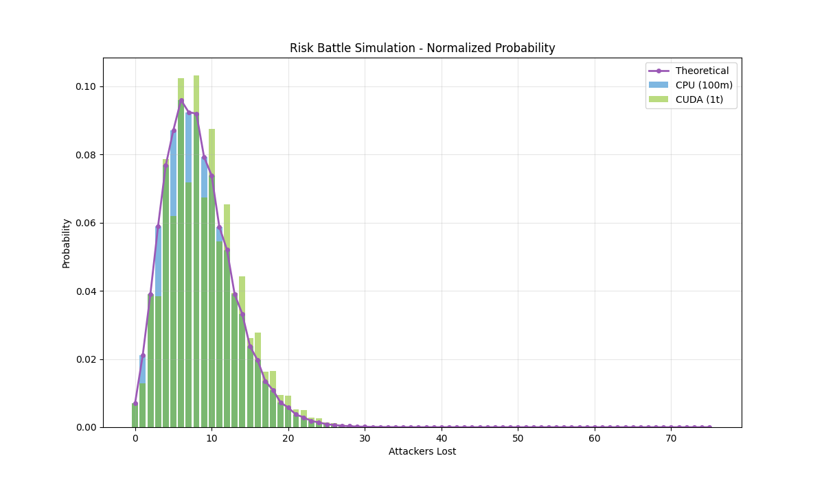
The theoretical curve peaks around 6-8 attackers lost with a characteristic asymmetric shape — notice how the slope alternates between steep and shallow steps, a direct consequence of Risk’s mechanics where ties (both sides lose 1 troop) occur ~34% of the time in 3v2 combat, while decisive outcomes (one side loses 2 troops) dominate the other ~66%.
The CPU simulation with 100 million trials tracks the theoretical curve remarkably well through the main distribution but lacks the sample size to capture outcomes beyond ~50 attackers lost. The CUDA simulation with 1 trillion trials extends deep into the tail, though it exhibits slight oscillations in the 4-10 range — likely a counting artifact in the histogram aggregation, as evidenced by the total summing to 1,000,000,192,512 rather than exactly 1 trillion. Despite this minor systematic error, both simulations validate the theoretical distribution: the probability drops below 1% after ~20 attackers lost and becomes vanishingly small beyond 25.
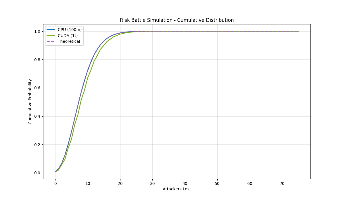
The cumulative distribution shows how quickly probability mass concentrates in the likely outcomes. All three approaches converge to essentially the same curve — by 25 attackers lost, we’ve accounted for over 99.9% of all possible outcomes. The CUDA simulation shows a slight deviation from the theoretical curve (visible as a small gap between the lines), consistent with the counting artifacts we saw in the normalized distribution. However, the deviation remains small throughout: the simulations successfully capture both the central tendency and the overall probability structure, confirming our random number generation reflects the true underlying distribution.
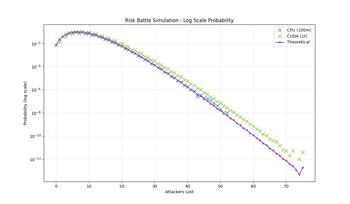
The log scale reveals the true test of our models: matching probabilities across 12 orders of magnitude, from common outcomes in the single digit percentages (
Notice the spike at 75 attackers lost, where probability jumps above 74 and even 73. This isn’t a bug — it’s real. That single data point represents the sum of 10 different defeat scenarios (ending with 1–10 defenders remaining), and losing with 1-2 attackers is actually more likely than barely winning when the dice strongly favor defenders at low troop counts. The aggregate of all defeat states exceeds the probability of any single “barely won” outcome.
The CPU simulation tracks the theoretical probabilities faithfully until around 40 attackers lost, where limited sample size causes it to overestimate the tail probabilities before disappearing entirely at 51 losses — it simply never observed outcomes beyond that point in 100 million trials. The CUDA simulation extends much further but shows systematic deviation: it undercounts outcomes in the 0-10 range (explaining the gap in the cumulative distribution), which compounds into progressively larger errors in the tail. Our initial observation of “4 defeats in 1 trillion simulations” turns out to be anomalously high — the true probability of losing all 75 attackers is
Question 2: What is the Expected Value for Troops Lost?
The simplest way to answer this question is to use our existing distribution which assumes starting at (75, 10). The expected value for a distribution is simply
Standard Deviation is a similarly useful metric to describe how much we can expect values to typically deviate from the expected value
The General Case
There are, however, some unique properties of 3v2 space we can use to come up with a more satisfying answer that isn’t dependent on our starting position.
First off — perhaps obvious but deserves being stated — the majority of dice rolls in a real Risk game occur in this space. An attacker is likely to stop attacking once they drop below three units, and if the defender drops below two they are usually one roll away from defeat.
Secondly, the edge traversal probability is uniform throughout this space. For example,
We’ll start by mirroring our implementation of constant_space_probability from Deriving the Common Case with a general formula that sums over possible counts of T-edges:
The multinomial coefficient
The Key Insight: Valid Paths Simplify Everything
At first glance,
These represent the number of
Recall from Deriving the Common Case that for any valid path,
- If both are even:
, so is also even - If both are odd:
, so is also odd
In either case,
Discovering a Constant
Let’s examine what
The total number of edges is constant across all valid paths! This allows us to factor out the multinomial coefficient’s numerator:
Reducing the Sum
Summing with a step of 2 is hostile to analysis, so we’ll make a k-substitution:
The bounds become:
For compactness, define:
so that:
Final Form
Substituting these expressions yields the cleanest general form (at least that I can come up with) for the transition probability in 3v2 space:
This expression depends only on the net troop losses and remains valid precisely because every term in the sum corresponds to a feasible path in the underlying state graph.
I’ll be honest: I don’t currently know how to push this expression all the way to the clean closed-form solution I had in mind. I can see the shape of what I’d like to do—extend the recurrence, analyze its limit as attackers grow large, and derive an exact expectation—but that’s a deeper mathematical problem than I have time to chase right now. What I can see is that the recurrence converges very quickly. Playing with the calculator above shows that for a fixed defender count of 10, the results stabilize fast: 20 attackers behaves almost identically to 70. Numerically, the expected attacker loss against 10 defenders settles around 8.3, which lines up nicely with both intuition and the simulation results.
Conclusion
What started as a grudge against a ridiculous game of Risk turned into a surprisingly deep technical exercise. I set out to answer a simple question—how unlikely was that disaster?—and ended up building a CUDA simulator capable of running a trillion battles in mere minutes (a feat I find disproportionate satisfaction in). The raw result was unambiguous: losing roughly 75 attackers against 10 defenders is an event so rare it appears only a handful of times in a trillion trials. Seeing it happen twice in a row remains, in purely probabilistic terms, absurd beyond everyday intuition.
The math provided a second perspective. By modeling battles with exact dice probabilities, I was able to sanity-check the simulation and estimate meaningful quantities like expected losses. While I didn’t push that analysis all the way to a closed-form solution, it converges quickly enough to confirm the big picture: against 10 defenders, an attacker should expect to lose only about 8.3 troops on average. My experience was not just bad luck—it was vanishingly, spectacularly bad luck.
More than anything, this project is a reminder that human intuition was never built for extreme probabilities. A calculator can produce arbitrarily tiny probabilities, but insight comes from understanding what those numbers actually represent. In this case, the answer is clear: sometimes the universe really does roll the worst possible dice—and occasionally it decides to do it to the same person twice.